Tracing the Evolution of Gas and Dust at Planetary Formation Scales using the Atacama Large Millimeter-submillimeter Array (ALMA)

Declaration

I hereby declare that the work in this dissertation titled Tracing the Evolution of Gas and Dust at Planetary Formation Scales using the Atacama Large Millimeter-submillimeter Array (ALMA) in partial fulfillment of the requirement for Masters of Science in Physics submitted to NISER Bhubaneswar is an original piece of research work conducted under the guidance of Dr. Liton Majumdar and Dr. Luke Robert Chamandy, NISER Bhubaneswar. This work was carried out in accordance with the requirements of the HBNI’s code of practice for research degree programs, and it has not been submitted for any other academic award. NISER is hereby granted the exclusive, royalty-free, non-transferable rights to make use of the dissertation for research purposes only, with appropriate citation.

Acknowledgements

I would like to express my deep and sincere gratitude to my supervisors Dr. Liton Majumdar and Dr. Luke R. Chamandy for their consistent motivational support. I extend my heartfelt appreciation to my lab (and batch-) mates Chandan Kumar Sahu and Dibya Bharati Pradhan for elevating the atmosphere with scientific rigour. I would also like thank my friend, Daksh Kadian, for being there for me during my time at NISER. I would also like to acknowledge the fruitful discussions I had with Baibhav Srivastava, Varun Manilal, Prathap Rayalacheruvu and Parashmoni Kashyap at SEPS regarding my project and the insights they provided. I would also like to acknowledge the constant emotional and mental support by mother provided over the course of this work. I would also like thank NISER, the SPS department for training me for doing research professionally. I specially thank the SEPS department for providing me the opportunity to conduct research in a professional lab environment, while treating me as a family member. At last, I thank Homi Bhabha National Institute and the Department of Atomic Energy for supporting me with the funding.

Introduction

Quote

“The stars, like dust, encircle me
In living mists of light;
And all of space I seem to see
In one vast burst of sight”

Isaac Asimov

Origins of Planetary Systems

Up until the 1990s, the only planetary system known was our own solar system and incidentally all theories on planet formation were primarily derived from its geophysical study [see @Brush1990 and references therein]. Things changed in 1990s after the discovery of the first exoplanet by @Wolszczan1992, shortly followed by the discovery of the hot Jupiter¹ 51 Pegasi b, the first exoplanet to be discovered orbiting a main-sequence star [@Mayor1995], and it was established that planetary systems are far more common that previously thought.

Study of how these planetary systems came to be is extremely multi-faceted and involved process and it is essential to narrow the scope to a particular epoch in the grand scheme of things. In nearby star-forming regions, most of the young stars (1 Myr of age or less), are surrounded by an optically thick circumstellar disk [@Williams2011]. The aim of this work concerns with these disks, which occur across stars of varying mass brackets, possess a thin-disk geometry with vertical extent no more than 10% to 20% of their outer radius, are composed of molecular gas and dust grains with sizes ranging from few microns to several mm [@Youdin2013]. We will outline the different methods that have been used to do this kind of modelling, and describe the kind of approach taken by this work in detail. But before doing that, it is essential to lay down the foundations of how protoplanetary disks themselves form and where are the seeds of planetary systems are truly sown in the chronological sense.

Diffuse and Dense Molecular Clouds

Life begins in death. Red giant stars towards the end of their life expell matter into the interstellar medium which eventually clumps together to form interstellar clouds, composed of gas, dust and plasma. A certain kind of interstellar clouds are of immense interest: molecular clouds. The qualifiers diffuse and dense refer to visual extinction and density of the regions respectively. These interstellar clouds are so referred to as molecular because their density and size permits formation (and sustenance) of molecular hydrogen. Within these molecular clouds, lie further clumped regions of even higher density, where star formation begins once the gravitational forces are sufficient to cause the dust and gas to collapse.

This collpase is what eventually leads to formation of circumstellar disks through the conservation of angular momentum during the formation of a star through gravitational collapse. In the beginning, although, the disk feeds material into the star, while simultaneously also being dissipated off to interstellar medium, with time, the accretion rates becomes steady and we are left with the disk, which will have a life time of few millions of years [@Williams2011].

The Laboratory Called Solar System

Our solar system is sole and closest place to verify and validate our theories on planet formation and for this reason, the importance of solar system science cannot be understated. For instance, minimum mass solar nebula (MMSN) [see @Desch2007 for a review] provides a simple estimate of the mass available in planet forming disks by distributing mass currenlty held up by solar system planets into concentric touching ring-like geomtries, and then adding volatile elements until the composition becomes solar. Variants of MMSN have been proposed by @Weidenschilling1977 [@Hayashi1981; @Crida2009-ef].

Besides getting constraints on mass, isotopic measurements of solar system objects that we can physically retrieve (such as meteorites) reveal formation conditions of the solar system. The significance of isotopes is revisited in the later chapters as well. Further, there is the question of origin of volatiles, specially water, on Earth and elsewhere like in comets.

The Cycle of Planet Formation

The process of planet formation begins with the collapse of a molecular cloud, resulting in the formation of a protostar and a protoplanetary disk around it. This disk is rich in gas and dust, and it is in this disk that the building blocks of planets are formed. Over time, the dust in the disk begins to coalesce into larger particles, which then collide and stick together to form planetesimals. These planetesimals continue to grow by accreting more dust and planetesimals, eventually forming protoplanets. The protoplanets can then undergo further growth and differentiation to form terrestrial planets, or they can accumulate large amounts of gas to form gas giant planets.

As the protoplanets continue to grow, they can undergo differentiation, with heavier elements sinking to the centre and lighter elements rising to the surface. This process can result in the formation of a metallic core and a silicate mantle, similar to the composition of the Earth. The protoplanets can also accrete gas from the surrounding disk, either through gravitational attraction or by forming a pressure gradient that draws in gas.

Ultimately, the fate of a planetary system is tied to the life cycle of its host star. When the star exhausts its nuclear fuel, it can undergo a supernova explosion, which can inject large amounts of heavy elements into the surrounding interstellar medium. These elements can then be incorporated into the next generation of protoplanetary disks, providing the raw materials for the formation of new planets.

Theories of Planet Formation

Planets are diverse and thus are the theories defining their formation. Giant planets which are mainly composed of hydrogen and helium, often dictate the orbital architecture of the planetary systems they form in due to theie sheer size [@DAngelo2018]. Two formation pathways for them have been extensively studied, first being the core accreted nucleation and other other being disk instability. For terrestrial planets, the picture is more uncertain and complex, with a chain of events that leads to formation of pebbles from dust grains, planetesimals from pebbles, planetary embroys from planetesimals and eventually planets from planetary embryos. For our inner solar system itself, there are multiple competeing as well as established theories like the Nice model [@Tsiganis2005]. The role of migration cannot be understated either, with theories like Grand Tack hypothesis in the fray [@Izidoro2018].

From Clouds to Disks to Planets

Protplanetary disks are the cradle of planetary systems. Understanding the evolutionary pathways that led to a planetary system like ours, which harbors the only planet to facilitate life, is of utmost importance. One of the most widely used technique to do so is physico-chemical modeling of these disks. The molecules present in these disks reveal themselves as we observe them through telescopes, present both in space and on the ground. This is achieved through spectroscopy of the radiation received to us from these distant objects.

Self-consistent Models of Protoplanetary Disks

Quote

“The scientific process has two motives: one is to understand the natural world, the other is to control it.”

C. P. Snow

Historically, the models used to study disks have been majorly of two types, with each having its own specialization. The first kind is the continuum or dust radiative transfer models like RADMC3D [@Dullemond2004], MCFOST [@Pinte2006] and MCMax [@Min2009] which specialize in performing a simulation to obtain (and later constrain) parameters like disk shape, dust temperature, dust-grain species (and their populations), radiation field and so on. The second is the chemical, or in some cases, thermo-chemical models, which include chemistry in varying degrees of complexity, along with UV and X-ray ionization, to explore the chemical properties of the gas and its temperature, with more emphasis on the outer-disk (less dense) regions of the disk as they can be traced by the (sub-) mm line observations.

With time, it has become evident that just the usage of one kind of these models does not suffice to make any new meaningful scientific inferences. Therefore, lately, all-in-one models like ProDiMo [@Woitke2009], DALI [@Bruderer2014] and rac-2D [@Du2014] or models which couple these two kinds of models have appeared to achieve some level of consistency.

Combining these different aspects of modelling is not straightforward as a lot of free parameters one would have to assume to move forward are themselves not very constrained (for example, the dust-to-gas mass ratio). The goal, ultimately, is to build a model, preferably self-consistent that handles all the aspects by itself, that can reproduce the observational data obtained by telescopes and eventually make congruous predictions on disk morphology and chemical observables. Because of the large number of free parameters, usually the models like these are computationally extensive, which further restricts the exploration of parameter space.

Modelling a Protoplanetary Disk

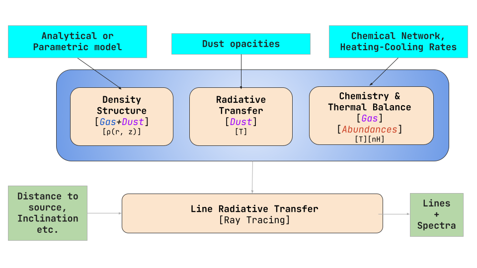
In order to draw any scientific conclusions from the observational data, we need to build forward models that can simulate the physical and chemical environments to a certain degree of accuracy in these planet forming environments. The chemical abundances which we can observe give a plethora of information on the underlying physical conditions. And likewise, the physical conditions (along with initial chemical make-up) we simulate can be tuned to fit the observations. Therefore, a disk model exists on the junction of the interplay between physics and chemistry.

These physical parameters include almost everything one can think about protoplanetary disks, from the disk morphology, to the nature of the interstellar dust regulating the disk dynamics, to the settling and the onset of coagulation of this dust into small pebbles that will eventually form planetesimals, initiating the process of planet formation. This dust, in turn is deeply coupled with the gas, which will later provide the raw material for gas giant planets. All of this, can be ascertained to a reasonable degree by studying the spectrographic signatures from these objects. The moment maps² of high spatial and high spectral resolution can reveal information on the disk gas kinematics, which can in turn reveal more substructure within these disks. Gas kinematics observations have even made detection of still-forming planets possible [@Pinte2019].

As the disk evolves, it loses mass through evaporation of gas and accretion on to the host star. Thus, the gas and dust also reveal information on the evolution and lifetime of disks. This sets the timeline for formation of those giant planets [see @Deeg2018]. The dust component in the disk, although usually only 1% of the gas, is also crucial, as it is what will form the terrestrial planets. Finally, the dust dynamics (involving dust growth, settling and inward radial drift) is heavily regulated by the gas content present in the disk.

Thus, from a modelling perspective two approaches can be taken, depending on the motivation. If the focus is on how material transforms in protoplanetary disks, then usually the spectroscopic point of view can be ignored, and instead, more emphasis can be placed on the different physical and micro-physical processes that couple the evolution of gas and dust and how can this interplay lead to formation of planets. Multiple works have incorporated a broad range of ideas to study from perspective, ranging from studying the effects of magnetic fields to models of pebble accretion. On the other hand, a spectroscopic or a chemistry-first point of view can be taken where the modelling is more concerned with the evolution of abundances of various interstellar molecules under varying physical conditions in the different regions of the disk.

To achieve this, we have developed a thermo-chemical disk model, which self-consistently couples the disk physics and disk chemistry. The model first does continuum dust radiative transfer whose output, the distribution of radiation field, is fed to the chemistry, where the model evolves abundances of various molecular species subject to a variety of chemical processes and a large chemical network. The physics and chemistry are coupled by considering the thermal balance of the gas, where different processes (physical or chemical) can heat or cool it, which ultimately leads to an energy exchange processe between gas and dust. As chemistry at any location is sensitive to the temperature, such a model becomes extremely crucial in our context. In the following sections, we will give an overview of the physics and chemistry included in our model.

Disk Dynamics

The disk dynamics can be formulated by starting with a mostly gaseous disk in orbital motion. Whether this motion is Keplerian or not depends on radial pressure distribution and usually this pressure support yields sub-Keplerian velocities. The equation of motion of such system can be succinctly written as

with representing the gas orbital velocity, being the gas density and being the gas pressure. The sub-Keplerian velocity now can be written in terms of Keplerian velocity as

where , the Keplerian velocity is given by and is the sound speed given by with being the adiabatic index.

But much more happens inside these disks than just plain orbital motion around the central star. Radial pressure gradients give rise to turbulence and pave a ways through which angular momentum can be transported from one location to another. And there can be different types of turbulences and instabilities according to their origin or progenitor. And all of this is extremely equivalent model planet formation as the regions where turbulence and transport are reduced and the gas decouples with prevalent magnetic fields in the disk, dead zones manifest where the planet formation processes start to take place.

Defining Traits of Disks

This section is chiefly about disk morphology and the traits which define a disk so that it can be modeled. The first and foremost is the surface density. We can only observe the disk averaged quantities and only models can help us to resolve the vertical structure in the case of non-edge-on disks. The other parameter of interest is the scale height, which are the measure of flaring in the vertical direction (which increases with radius). This is also related to concept of dust settling implcitly as both together can give a better idea of how the material is distributed through the vertical structure. Finally, azimuthal symmetry is a convenience that is often assumed which might not be necessarily true always. Asymmetries imply additional influences, which can sometimes mean still-forming proto-planets.

The Interplay of Physics and Chemistry

A Chemical Viewpoint

It is evident that protoplanetary disks can be studied both from a dynamical perspective and from a spectroscopic perspective. This work leans towards the latter in the sense it utilizes chemical modeling of these objects instead of numerical modeling of orbital dynamics and fluid mechanics. In the end, for the complete picture, it is essential that all things must be considered and validated for consistency but the former falls out of the scope of the current work.

Astrochemical Reaction Networks

Chemical networks are list of reactions with their respective rate-coefficients, and suitable physical conditions, that can take place in the interstellar clouds (and disks). The physical environments in clouds and disks are diverse. If one assumes three stages of planet formation, various physical conditions can be tabulated as in Table [tab:my-table1]{reference-type=“ref” reference=“tab:my-table1”}. There are several well-established networks published in the community for planet formation environments like UMIST (with the most recent release published being @Millar2024) and KIDA (latest release being @Majumdar2016). For our intents and purposes, which are described in later chapters, we have used the latter.

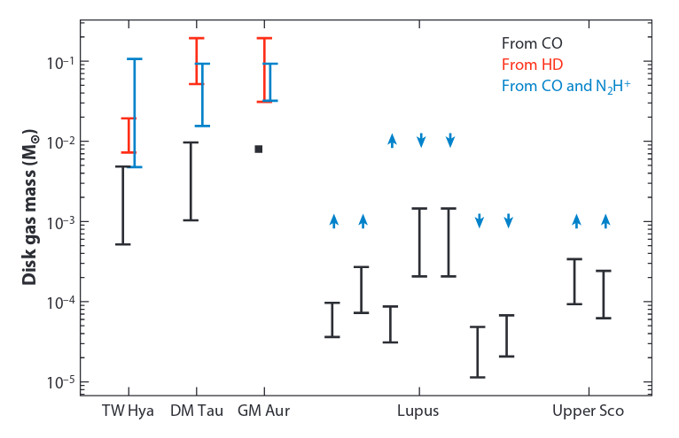
What Can Disk Mass Tell Us?

We have seen that, in all sense, the physical parameters we can constrain for the protoplanetary disks are mostly rooted in understanding their chemical composition. The gas mass of the disk is no exception. The importance of constraining the gas mass is many-fold @trapman2022novel; with the most evident being that the gas is the reservoir that will provide the raw material for gas giant planets to form. As the disk evolves, it loses mass through evaporation of gas and accretion on to the host star. This sets the timeline for formation of those giant planets (see @mordasini2018handbook). The dust component in the disk, although only 1% of the gas, is also crucial, as it is what will form the terrestrial planets. The dust dynamics (involving dust growth, settling and inward radial drift) is heavilty regulated by the gas content present in the disk @birnstiel2012simple.

However, obtaining an estimate on disk gas masses has been proven to be arduous. Hydrogen molecule () is the chief constituent of the gas so if we can constrain the abundance of in disks, it will provide an excellent idea on the total gas content. But due to absence of any dipole moment, it does not emit significantly in the temperatures found in the disks ( K). We have hydrogen deuteride (), which traces hydrogen gas chemically @trapman2017far, but it emits in far-infrared and currently, due to an absence of a capable far-infrared facility in the post-Herschel era, making it virtually impossible to make any observations of it. The next most abundant species in disks is carbon monoxide () and emissions from its isotopologues have been the subject of study for a plethora of work (see @Zhang2017 [@Booth2019] to name a few).

Although is assumed to have a relative constant abundance (relative to , denoted by ) in the warm gas of the disks due to its chemical stability of around @trapman2022novel, it can deplete from the gas due to photodissociation in the upper layers of the disk through irradiation by FUV photons or through freeze out the dust grains in deeply shielded, cold mid-plane of the disk @vanDishoeck1988 [@vanZadelhoff2001; @Visser2009; @Miotello2014]. These processes have been incorporated in physicochemical models and corresponding gas mass measurements have been made by reconciling the model results with the observations of and line fluxes @Williams2014 [@Miotello2016].

However, when these gas masses were compared to the ones derived independently from , the -based gas masses were found to be underestimating the result by several factors of magnitude (see @Favre2013 [@Kama2016; @McClure2016; @Schwarz2016; @Trapman2017; @Calahan2021]). This is suspected to be caused by either some chemical processes depleting in the gas or dynamical processes like grain growth trapping the ice-deposited dust grains. Thus, to measure reliably, we need to look for species which can serve as calibrators of abundance.

One such calibrator was studied by @trapman2022novel in the form of . The following reactions are of interest:

It is evidently clear that can only be abundant if there is a lack of . But this is only one such example, there might be several others, and it is a function of the breadth of the chemistry that a model has considered. Here, the term chemistry encapsulates both the number of reactions considered (the chemical network) and the different types of chemical reactions that can happen in the warm gas of these transition disks. The aim of this thesis is two-fold: to perform a statistical study across grids of forward theoretical disk thermochemical models to identify calibrators like these which can be detected by the current state-of-the-art observatories like the Atacama Large Millimeter/submillimeter Array (ALMA) and to include isotope chemistry @Majumdar2016 to model for species like considering the future observational missions like the PRobe far-Infrared Mission for Astrophysics (PRIMA).

Line Diagnostics

Once a simulation is done, the data produced by it has to be converted into form of something which telescopes will observe. Our code is accompanied by a ray-tracing module which performs line radiative transfer in a two-step process @Kamp2010. The first step is to solve the level populations for a given molecule. If sufficient information on its collisional parteners is available then the level populations are solved in non-LTE ³, otherwise the calculations are done in LTE. The next step is to perform the ray tracing by solving the transfer equation @Pontoppidan2009

where the source function is given as

The superscripts and refer to continuum and line emissivity functions and opacities.  is the macroscopic velocity projected on the ray. Once done, it is possible to generate emission maps of the source modeled with the help of additional parameters like inclination and distance to the source.

The Physical Structure of a Protoplanetary Disk

Quote

“Measure what can be measured, and make measureable what cannot be measured”

Galileo Galilei

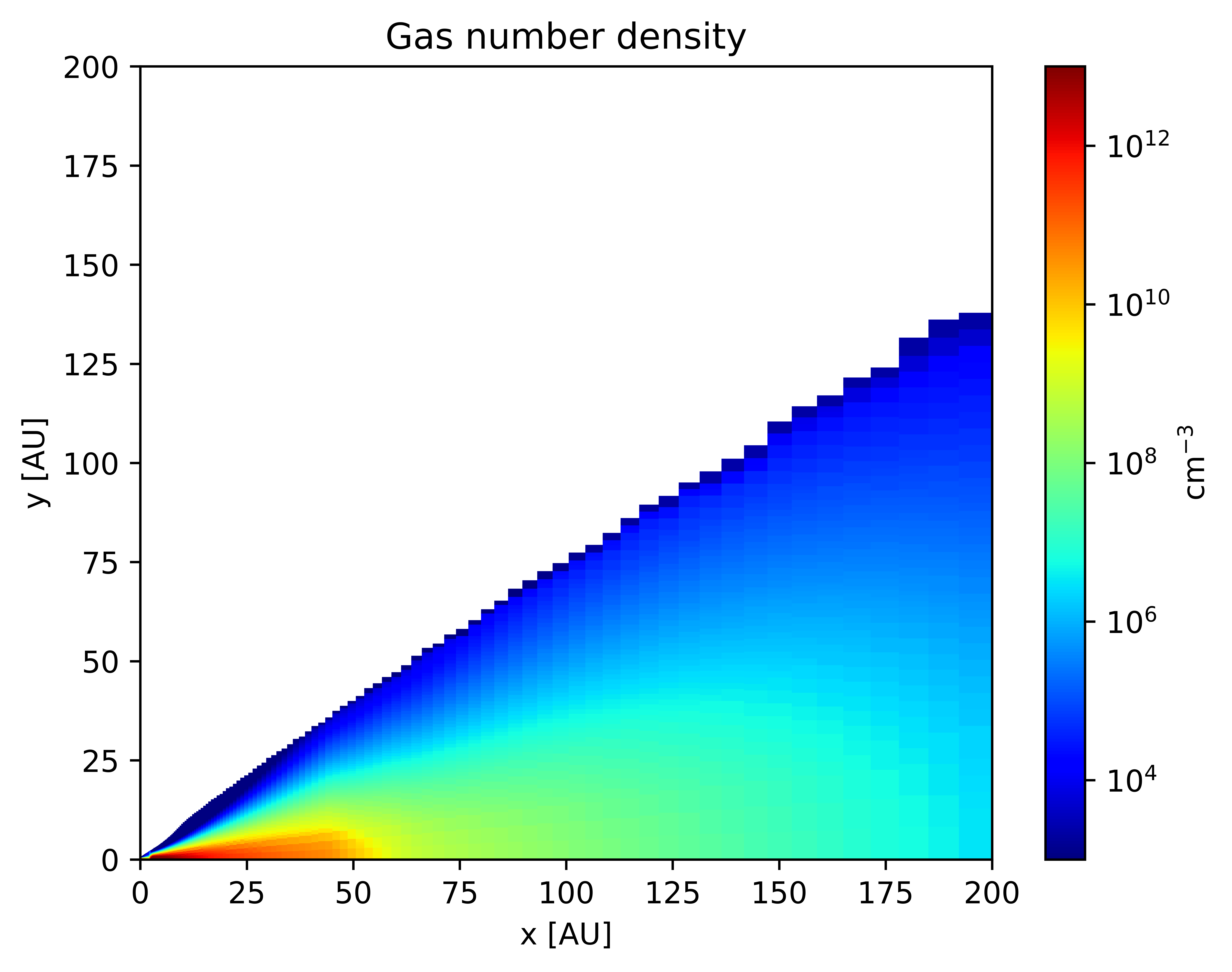
The Density Profile

The physical structure of our model is similar to as described in @Du2014 and @Woitke2009. This disk is assumed to be axisymmetric. We start with a parametrized distribution structure in cylindrical co-ordinates for the gas number density following  @lynden1974evolution [@Hartmann1998; @Andrews2009; @Cleeves2013] as an observationally constrained equation of the form:

where is the surface density by

is the characteristic or reference radius for which observationally constrained surface density is known. This is a constrain in the radial direction and likewise in the vertical direction, we have

where representing the scale height at . Scale height of the disk provides a measure of “flaring” in the disk, which is to say, the amount the disk rises relative to the mid-plane as we traverse further out radially.

The disk gas (or dust, as dust is assumed to trace the gas with 1% of its abundance) mass can now be found by integrating from inner edge to outer edge.

We begin by taking as an input through which we get the value of to get .

Further, we follow the gas temperature structure from @Williams2014 given as:

Hydrostatic Disk Structure

Our disk is static in the vertical and radial direction but in Keplerian rotation in the azimuthal direction, around the -axis. From the hydrostatic equations:

Here, is the velocity in along the azimuthal direction and is the gas thermal pressure, with being density. We neglect self-gravity, which gives the gravitation potential as:

where is the stellar mass and is the Newtonian gravitational constant. We assume that the radial and vertical components of equation of motion are independent of each other as the radial pressure gradient () is insignificant in comparison to centrifugal acceleration and gravity, allowing us to get the Keplerian velocity of our disk:

Getting this velocity is crucial as it is used while doing ray tracing to construct the observables from the modeled disk.

Dust Settling

As the disk evolves, the dust grains settle down in the midplane due to gravity. This process is much more apparent for larger grains, and in general the simultaneously ongoing process of dust growth will always lead to settling of these now heavier particles. Eventually, these initiate the formation of planetesimals, and in our context, are extremely important to model because they can trap volatiles like into them. Although our model does not explicitly and self-consistently consider the settling process (like done by @Dullemond2004b [@Dullemond2005]), we replicate the process through two pathways. The first involves decreasing the total dust mass within the disk while maintaining a consistent dust-to-gas mass ratio throughout, and the second entails diminishing the scale height of larger grains. In the second approach, a mixture of small grains with gas is retained, ensuring that the overall dust-to-gas mass ratio aligns with the standard model.

Thi parametric appraoch involves calculation of following dimension-less factor

where is the gravitational constant, is the stellar mass is the mean molecular mass of the cell, is the proton mass and thus the numerator represents the mass of the cell as it rotated arounds the star at a distance .  is the Boltzmann constant and the whole fraction is multiplied by the vertical extent of the cell. Combining them from a pair of neighbouring vertical cells we then calculate

This is calculated for every pair of consecutive cells ( being the upper cell) in the vertical direction and the gas number density of the top cell is scaled like

An alternative approach is also implemented where the gas thermal pressure is used to calculate the rescaling factor of the gas number density.

The settling plays an important part in finding a converged physical structure of the disk. By convergence, we mean that the and for a cell are within some permissible value. As comes from the Monte-Carlo radiative transfer and , an iterative approach is taken. This iterative approach allows to mimick the spectral energy distribution to suitably high precision. Furthermore, because the radiative transfer is parallelized, this process is preferred over a non-settled and a non-converged physical structure.

Continuum Radiative Transfer

Once we have setup the dust in our model, we can now create a grid which will be the stage for the simulation of our disk. Note that that equations  ![!insert ref] are for gas, but as already states dust follows the gas, with 1% of its abundance. The choice of the grid is extremely important, as the this grid is going to be used to simulated photon transport in a medium. As our disk is axisymmetric, it is enough to model one quadrant in 2 dimensions, with the source of photons (that is, the host star) athe origin. Many models often use a normal polar or cartesian grid but these density distribution require a finer (or adaptive) treatment where the grid scales accordingly (finer in dense regions and sparse in regions with low density). Therefore, as already described, we adopt a tree-based grid, which allows us to employ an adaptive resolution and easy to program ray propagation along the grid. This grid also allows a more accurate treatment of calculation of observables as we are not bound under the assumption of light/radiation propagating in a straight line, rather we can propagate an actual physical ray through our grid and any integrations along the ray path will be more closer to reality.

Monte Carlo based photon transport

The central star emits photons photons and they propagate through the disk where we only assume dust to be present (only for the radiative transfer run). The fundamental concept involves partitioning the luminosity of the radiation source into equally energetic, monochromatic photon packets. These packets are emitted in a stochastic manner by the source and are subsequently tracked to random interaction locations determined by the optical depth. At these locations, the packets undergo either scattering or absorption, the likelihood of which is dictated by the albedo. In the case of scattering, a random scattering angle is derived from the scattering phase function (differential cross-section). These is the same Monte Carlo based dust radiative transfer strategy described in @bjorkman2001radiative.

Let the stellar luminosity be which we divide into photon packets each with energy giving Upon injection into the disk (grid), the monochromatic photon packet will be assigned a frequency at random, selected from the spectral energy distribution (SED) of the source. The dust we have setup in our disk can now scatter, absorb or reemit the incoming radiation. All of these processes require us to have the opacity of the dust in our model, which depends on its composition. We have considered graphite based and astronomical silicates but we optical data for other dusts like pyroxenes as well. All of this data is taken from @draine1984optical. The frequency of the incoming photon packet in a grid cell determines the corresponding opacity. If a packet is absorbed in the cell, we deposit its energy (given by where is the number of packets absorbed by that cell ) to the cell and recalculate the cell’s temperature. As the cell is assumed to be in local thermodynamics equilibrium, the absorbed energy must also be reemitted. The emissivity of dust can be written as

where is density of the cell and is the Planck’s function at temperature . Therefore, we can write the emitted energy as:

where is the Planck mean opacity given by

with being the integrated Planck function. If cell had temperature we can write

where is the mass of the cell. Finally, equating [eq:mc4]{reference-type=“ref” reference=“eq:mc4”} to the energy absorbed by the cell, we get

[]{#eq:mc5 label=“eq:mc5”} One way to solve equation is through some iterative algorithm but we instead create a look-up table to speed-up calculations for each frequency/wavelength.

Thermochemical Evolution

Quote

“Chemistry begins in the stars. The stars are the source of the chemical elements, which are the building blocks of matter and the core of our subject”

Peter Atkins

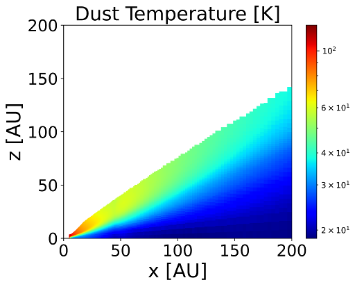
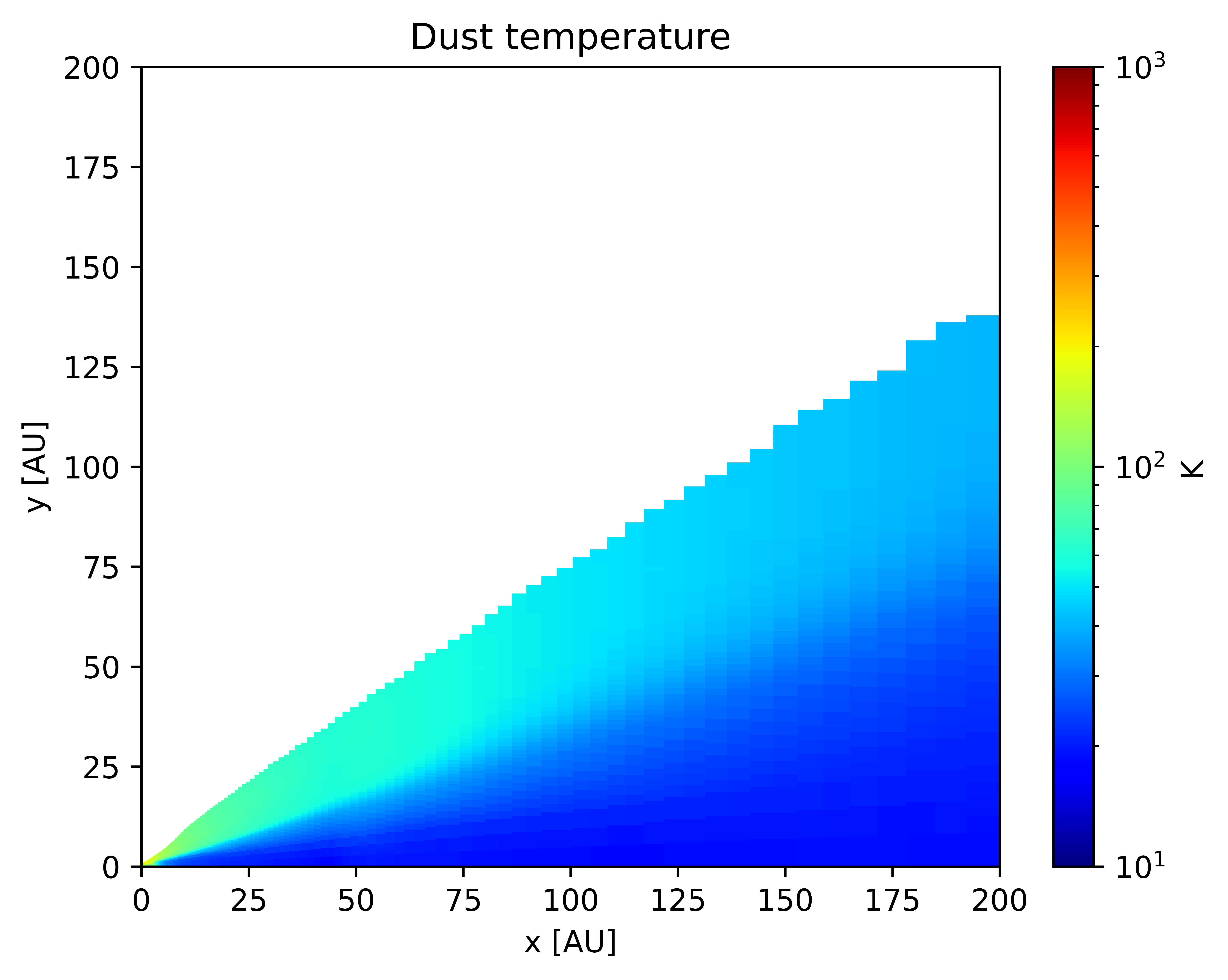
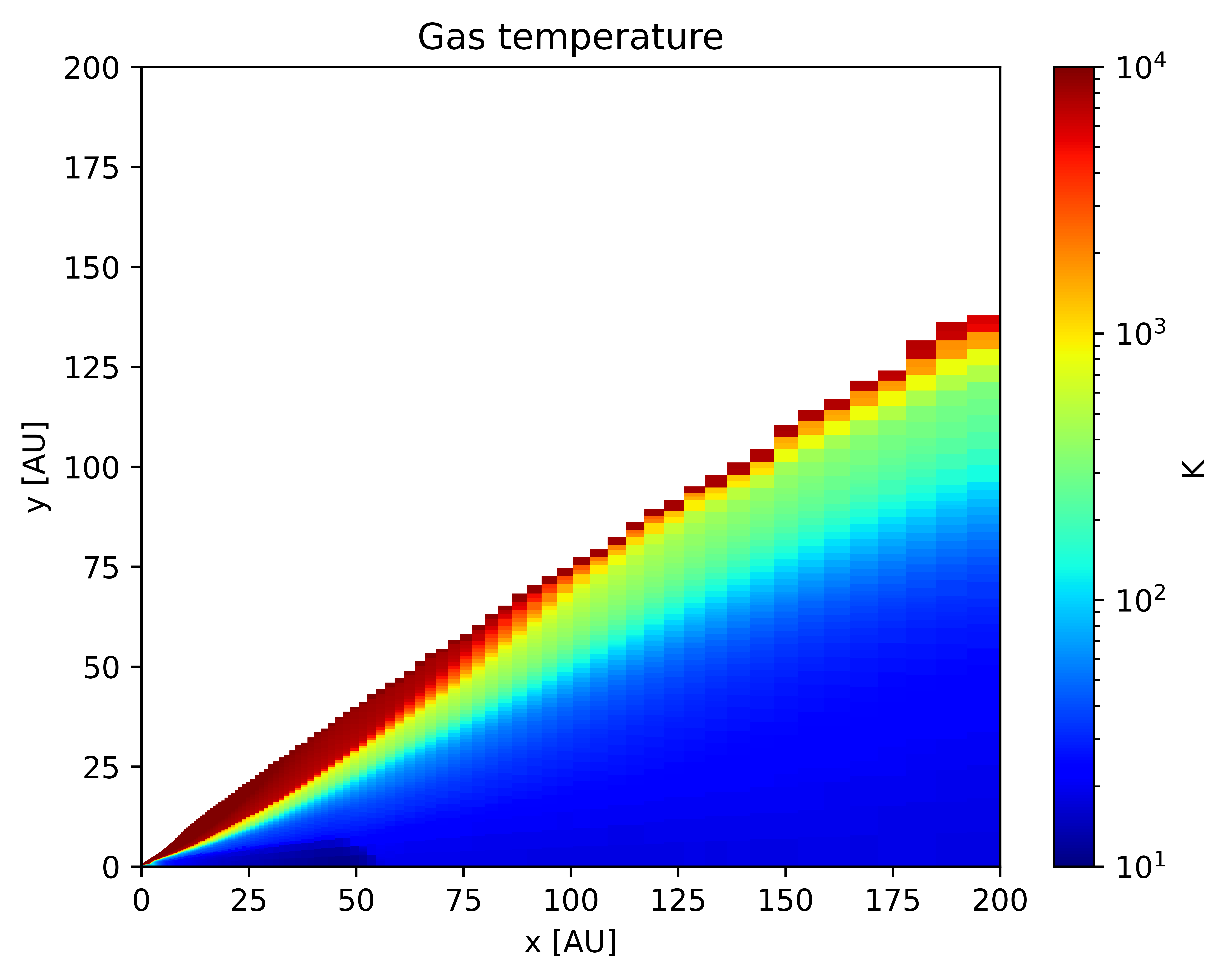
Once the dust radiative transfer is done, we will have obtained the dust temperature structure as well (see figure [4.1]). This will serve as the input to the chemistry, along with a set of initial elemental abundances, which are derived from observational constraints on the chemical make-up of the interstellar medium.

This section describes the various chemical processes and heating and cooling sources we have included in the model.

The Essence of Thermochemical Modelling

To self-consistently evolve the gas temperature along with evolving abundances, we need to consider the processes which can increase or decrease the temperature of the gas. The various heating and cooling processes we consider are photoelectric heating due to small grains and polycylic aromatic hydrocarbons (PAHs), heating and cooling from the energy released through exothermic chemical reactions, heating by the formation of , heating by viscous dissipation, heating by cosmic-rays and X-rays, energy exchange processes through gas-dust collisions, heating by photodissociation of , , , heating by ionization of atomic carbon, cooling by electrons recombining with small dust grains, cooling by rotational transitions of and rovibrational transitions of and , heating and cooling by vibrational transitions of , cooling by and emissions and cooling by Ly emissions.

We used the KInetic Database for Astrochemistry (KIDA) as the provider for our chemical network.

The equation we solve is given by where is the abundance of species , and being the production and destruction rates. and represent the heating and cooling rates respectively. We employ the use of SciPy [@2020SciPy-NMeth] library’s LSODA solver which is based on legacy solver of the same name.

Three-phase Gas-grain Astrochemical Models

As described earlier, to identify new chemical disk gas mass tracers, we need to explore the chemistry across vast parameter space. This includes inclusion of all the possible chemical processes that can explain the observation of certain molecule that we might have already detected in disks. If we are able to include all the major pathways that can lead to the formation (or destruction) of the species of our interest and it fits the observations well, then the whole process becomes a lot easier. Note that our chemistry is the so-called three-phase chemistry, with the three phases being the gas phase, the surface phase (species deposited on a grain surface in form of ice, free to react with species in the gas phase) and mantle phase where the species is trapped inside the grain after being covered up with more layers of accreting chemical species.

We adapt our chemistry from the work described in @ruaud2016gas. The reactions types we have included are the gas phase reactions with grain surface, formation of on grains, photodissociation and photoionization by cosmic rays, X-rays and cosmic-ray-induced UV photons, bimolecular reactions in gas phase, thermal desorption or evaporation from the grain surface, cosmic-ray desorption or evaporation from the grain surface, accretion on the grain surface, photodesorption by external and cosmic-ray generated UV photons, photodissociation by cosmic-rays and UV photons on grain surfaces, grain surface reactions, swapping between grain surface and grain mantle, the Eley-Rideal mechanism (where a gas species approaches a grain surface species and forms a product which remains on the grain surface).

For bimolecular reactions, we employ the modified Arrhenius rate equation But for reactions involving a ion-polar reactants, a slighlty different approach is used where the reaction temperature range introduces a modification. As the temperature is also evolving with abundances self-consistently, the ion-polar reactions are extremely crucial.

Chemical Kinetics in Clouds and Disks

Our astrochemical kinetics models was extended from a 0-D model originally designed to model molecular clouds. This extension to a 2-D geometry requires consideration of few things. Pertaining to the physical parameters required to solve chemistry at each grid point, the order in which they are solved becomes important. This is because the attenuation of radiation along any direction has to be considered to calculate the rates of reactions like photodissociation from UV photons. Abundance molecules like molecular hydrogen and carbon monoxide can shield other molecules (and themselves) and to find the factors which can quantify this shielding, we need to propagate a light ray in the direction of incoming radiation upto the point where we are interested in solving the chemistry. Because the abundances will now influence how much radiation gets attenuated, which is not constant, it is impossible to solve all grid points simultaneously. Therefore, we adapt a different approach by starting at a grid point present at the disk surface at the disk inner edge. No material lies above it (and thus the incoming radiation from ISM will not be attenuated) and the central star. Then, we solve for the grid point directly below it. And this process goes on until we reach the grid point situated at the mid-plane. After this, we repeat this process for the next column, or more aptly, the next radial point. Therefore, the whole global iteration follows this order of top to bottom, in to out of solving the chemistry which takes the shielding of radiation into account accurately.

The chemical processes considered in our model are: gas phase reactions with grain; formation on grains; photodissociation and photoionization by cosmic rays, X-rays and cosmic-ray-induced secondary UV photons; bimolecular gas phase reactions; thermal desorption and evaporation; cosmic ray desorption and evaporation; accretion on grain surfaces; photodesorption by external and cosmic ray-generated secondary UV photons; photodissociation by cosmic rays and UV photons on grain surfaces; grain surface reactions. and the Eley-Rideal Mechanism.

Alongside the chemical processes, we also have following heating and cooling processes: photoelectric heating due to small grains and polycyclic aromatic hydrocarbons; heating by formation; heating by viscous dissipation; heating by cosmic rays and X-rays; heating by photodissociation of , and ; heating by ionization of atomic carbon; cooling by electrons recombining by small dust grains; cooling by rotational transitions of H2, and rovibrational transitions of and ; cooling by Lyman-Alpha emissions; chemical heating and cooling; heating and cooling by vibrational transitions of , and cooling by and emissions and everything is then connected through the energy exchange between gas and dust.

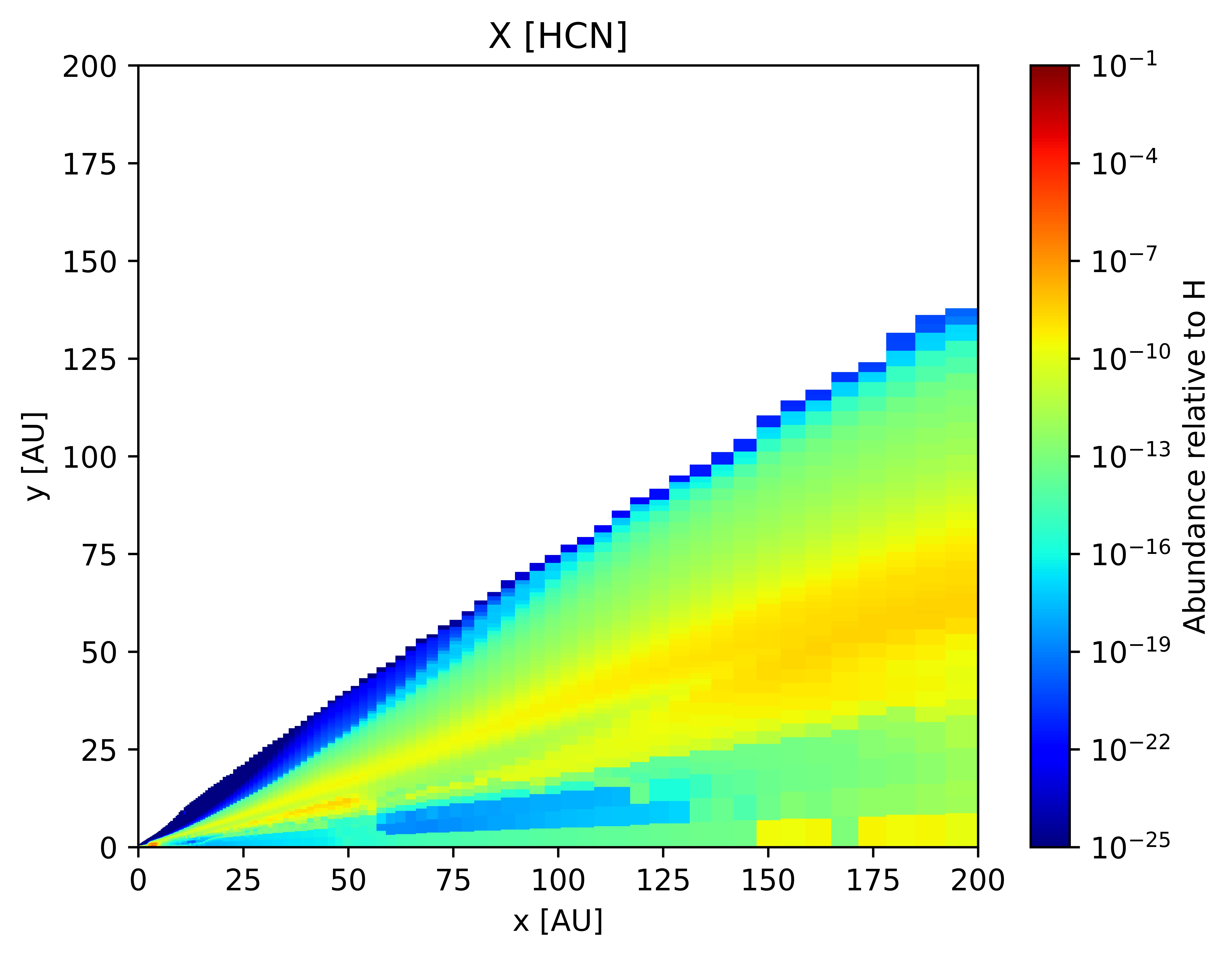
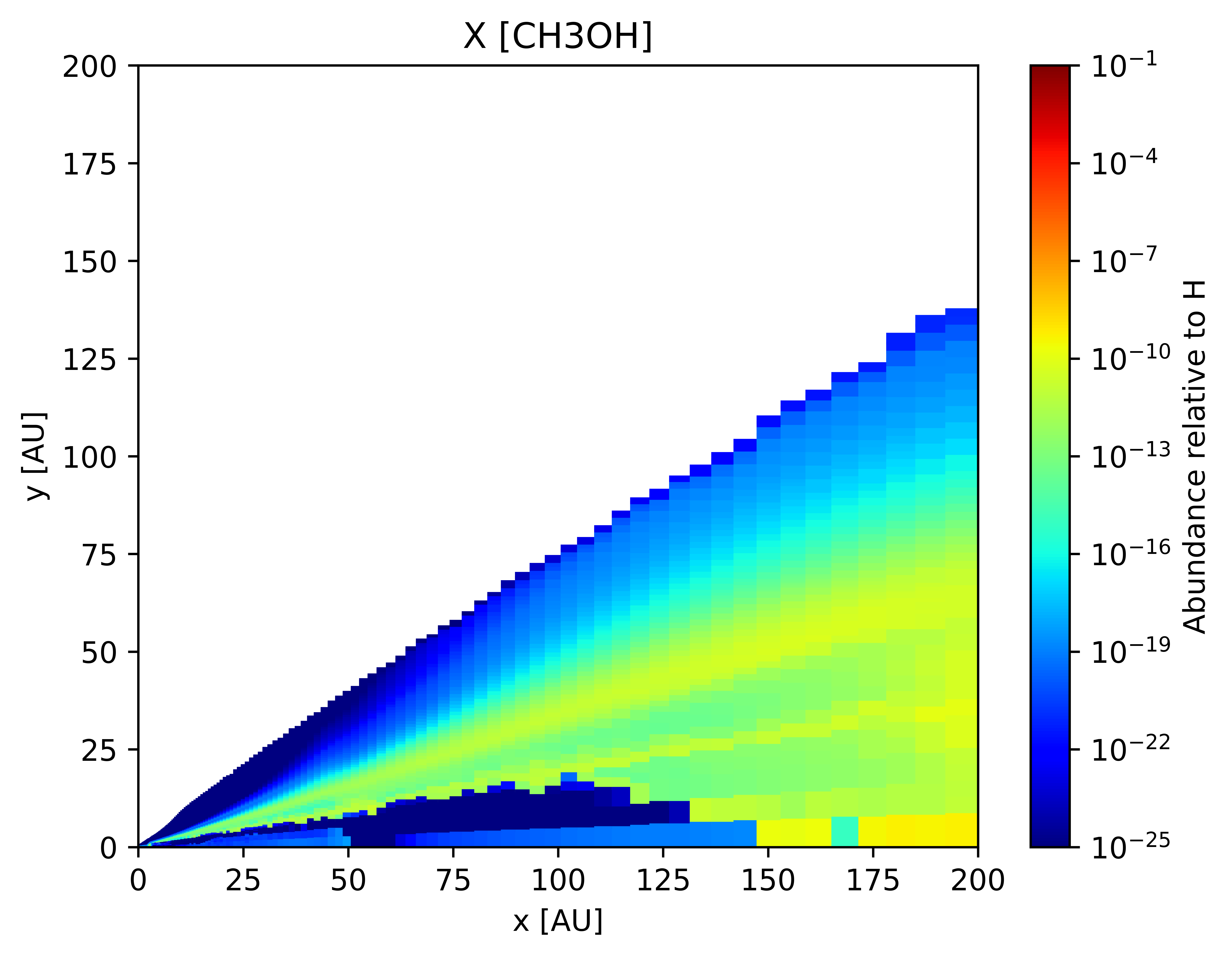
Ices and Snowlines

The distributions of volatiles in disks, including volatile organics, provide the initial conditions for planet volatile compositions and chemistry. The radius beyond which a volatile can only exists in form of ices, deposited on the dust grains, is referred to as the snowline of that particular volatile. These locations hold significance for several reasons. Firstly, the freezing out of key volatile substances alters both the chemical processes in gas and on grain surfaces. For instance, the freezing of CO facilitates the creation of oxygen-rich organic compounds in ice and could encourage carbon-rich organic chemistry in the gas phase. Secondly, in models of planet formation, the snowlines of major elements such as oxygen, carbon, and nitrogen dictate the volatile compositions of planetary atmospheres and envelopes, providing a key framework for understanding the atmospheric compositions of observed exoplanets. Thirdly, snowlines, particularly the water snowline, are anticipated to influence the evolution of dust grains and could regulate the timing and location of planetary core formation, thereby influencing whether terrestrial planets, Neptune-like planets, or gas giants form in certain regions [@berg2023].

On the Significance of Isotopes and Spin isomers

The isotopogues of a molecule are often opticall thin then the stable counterpart. The origin of isotopic fractionation lies in the fact that the zero-point energies dictate that the heavier nuclei will be more stable at low temperatures. These isotopic distribution patterns then can be used to assess the current thermal or irradiation environment or to link together different evolutionary phases [@Ceccarelli2014]. Similar is the case of spin isomers of species like hydrogen, ammonia and water.

Results

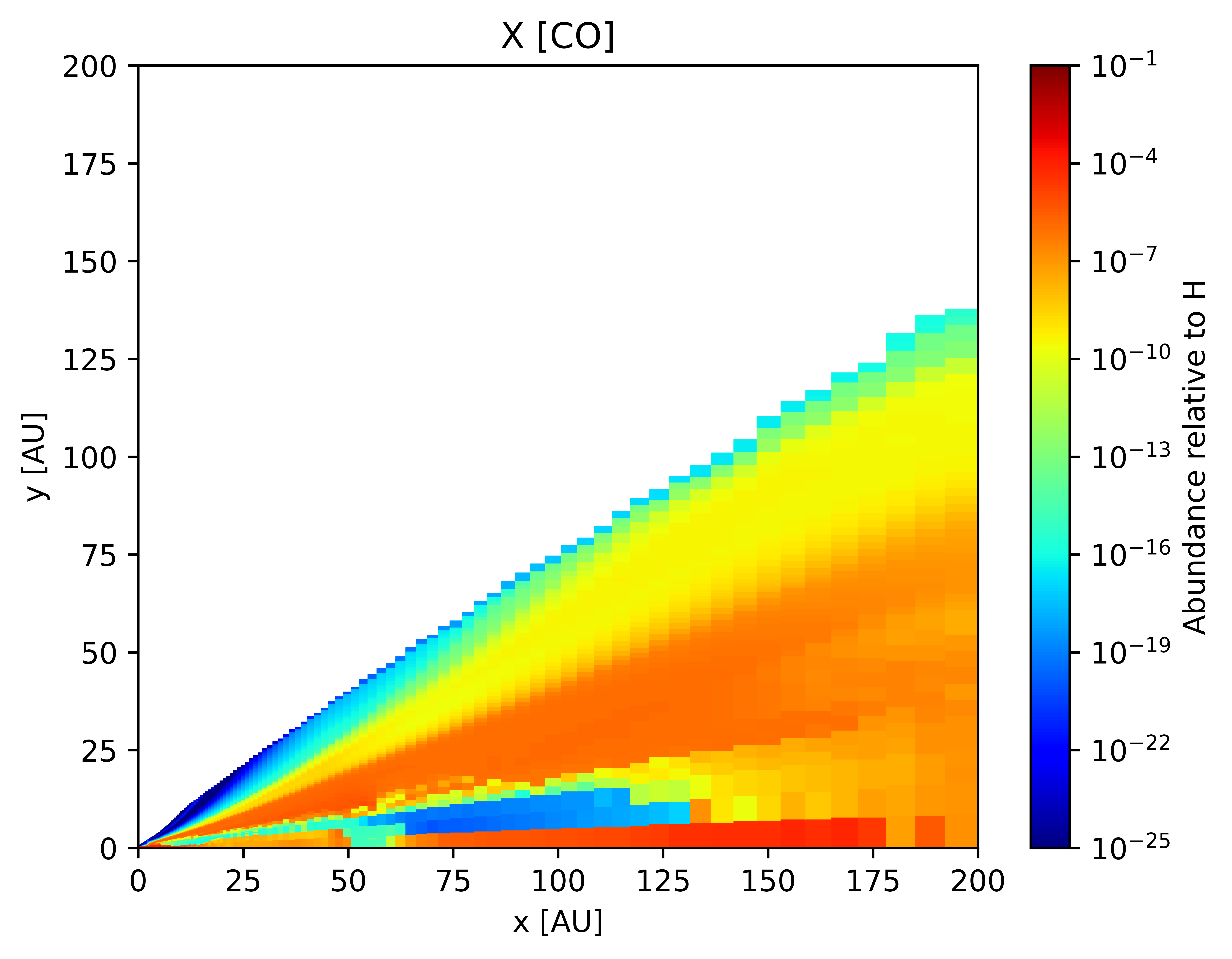
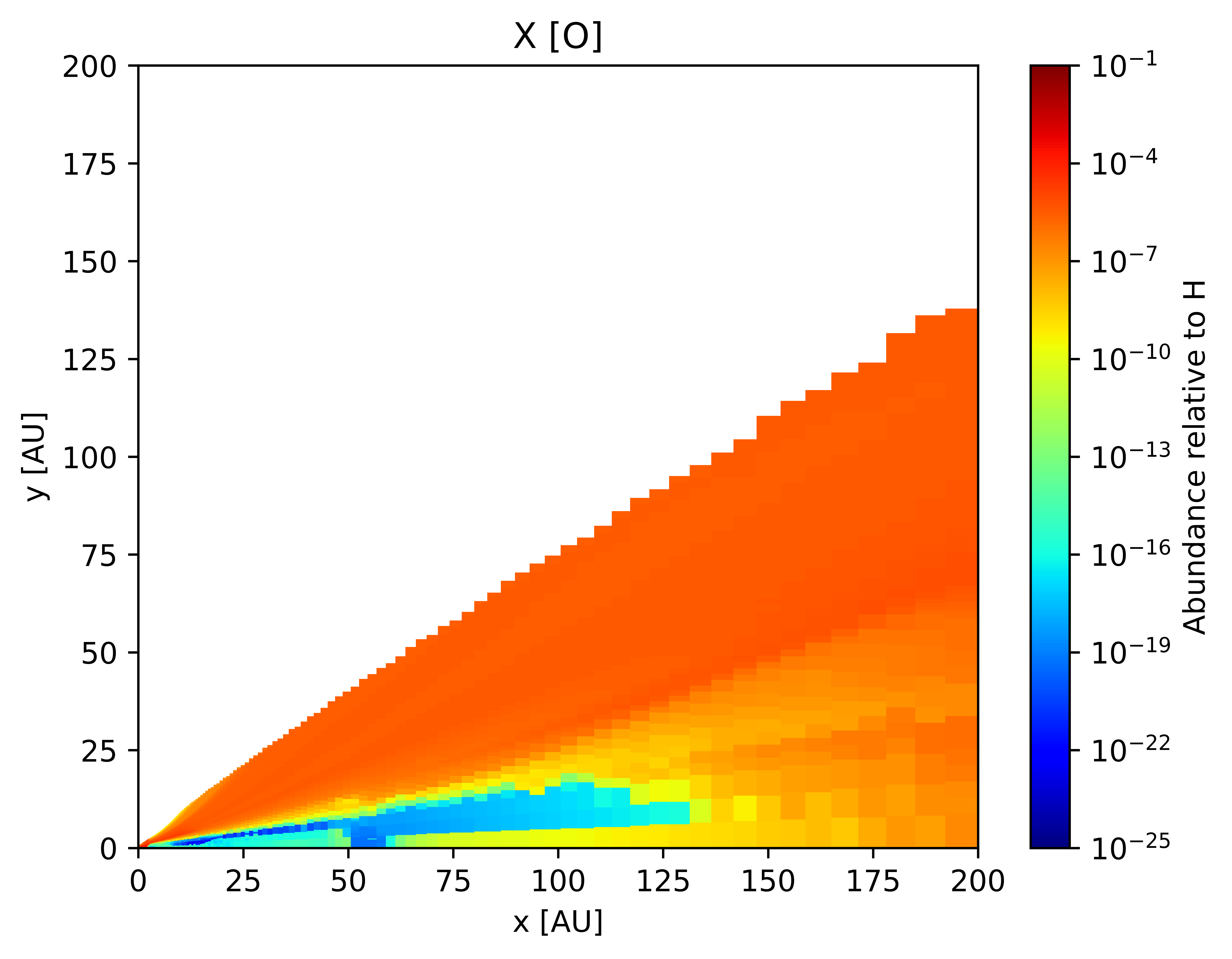
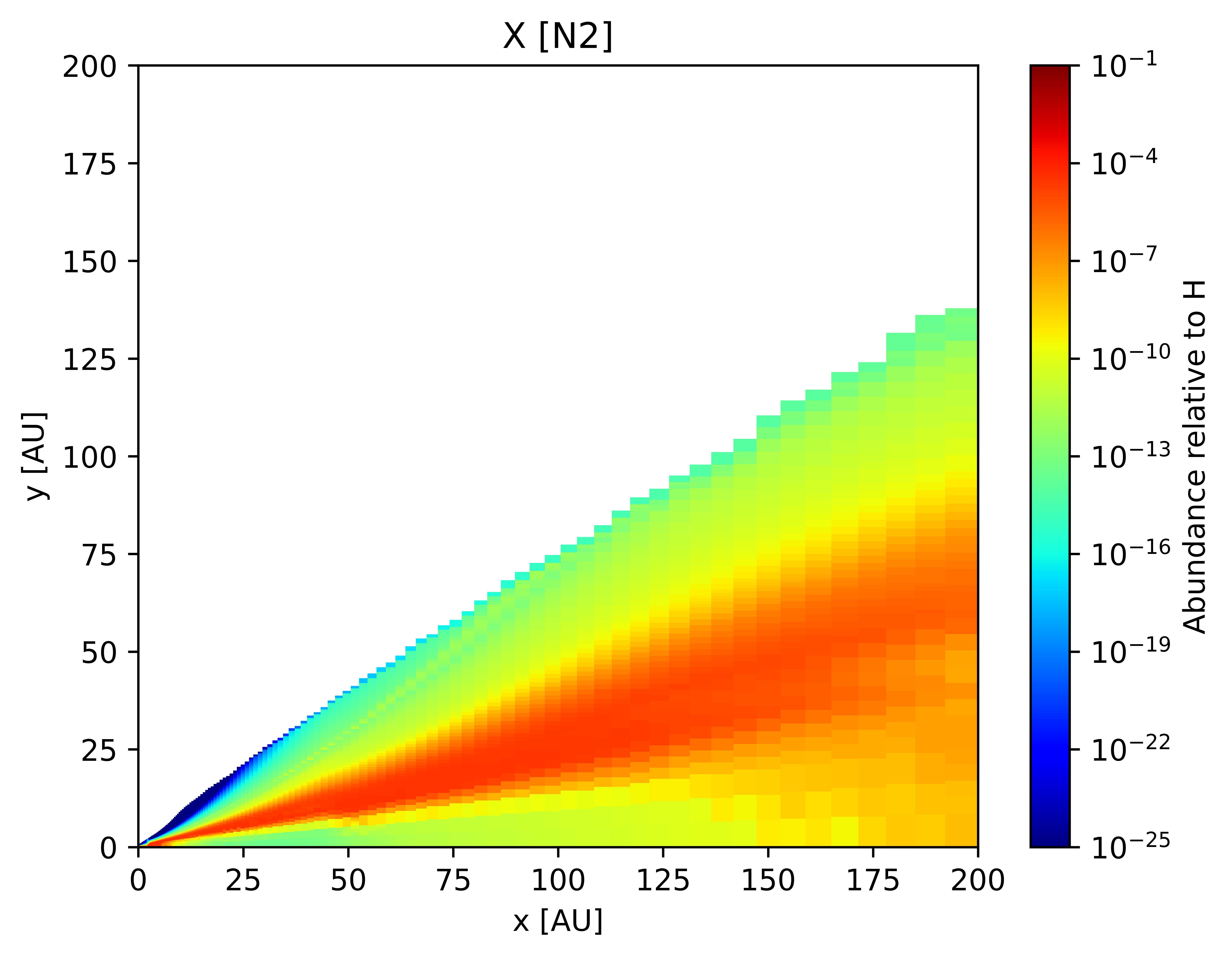
In this section, we present select results after a full thermo-chemical run from our model for a typical T-Tauri disk.

Simulating Observations

Quote

“The history of astronomy is a history of receding horizons”

Edwin Powell Hubble

The Theory of Ray Tracing

After the thermochemical calculations are done, we are in position to generate the observables that will mimic observations from telescopes. But even before that, we need to perform line radiative transfer to identify how would the radiation (line emission) look like given the distribution of a certain chemical species in our simulation using the technique of ray tracing.

Ray tracing is a fundamental method employed in the simulation of protoplanetary disks, aimed at delineating the trajectory of photons across a volumetric grid. This process entails a meticulous assessment of the interactions between photons and the constituent dust and gas within the disk environment. Paramount to the fidelity of such simulations is the acquisition of precise data pertaining to various physical and chemical attributes. These encompass crucial metrics such as the abundance and distribution of pertinent molecular species, dust densities, gas kinematics, and spectroscopic insights into molecular transitions of interest. Through meticulous consideration of these parameters, it becomes feasible to generate a comprehensive array of primary observables, encompassing line emission profiles, continuum and line emission imagery, moment maps, and channel maps, thus facilitating a nuanced understanding of protoplanetary disk dynamics. There are many techniques of doing ray tracing in context of protoplanetary disk models, like the “Long Characteristics” (LC) method where integrations are performed by constructing a large number of parallel rays passing through a given density structure at different impact parameters @Pontoppidan2009.

Visualizating simulations

Once simulations are complete, there are a varity of visualizations that can be made that are very relevant to what is observed. Once particular lines are resolved, a lot of information can be extracted. Interferometric data is typically presented in a data cube format, consisting of two spatial dimensions and one spectral dimension. To visualize this data effectively, researchers commonly employ 1D or 2D slices through the cube. Apart from examining the spatially integrated line profile as discussed earlier, various other visualizations such as moment maps (spatial maps), channel maps (velocity channels), and position-velocity diagrams (along one spatial dimension) can provide valuable insights [@Kamp2010]. Moment maps can be constructed for velocity integrated intensity (zeroth moment), intensity-weighed velocity (first moment) and intensity-weighed velocity dispersion (second moment). We can also make position-velocity diagrams to get an idea on determination of the disk inclination and the detection of infall/outflow or warps.

There are also channel maps which can reveal substructures within disk.

Summary and Outlook

These are the future directions for this project:

1. This work was a in-depth look into the modelling of protoplanetary disks through a holistic all-in-one thermo-chemical model.

2. Our thermo-chemical model has been successful in reproducing the results similar to established models. Beyond benchmarking, it has also improved upon various aspects of models and codes before it. Apart from being highly modular and written in a high-level language like Python, it is extremely performant due to use of JIT compilation through the Python library numba.

3. It’s radiative transfer module is parallelized and one of its kind in the treatment of how work is distributed among different CPU threads. Instead of doing parallel transport of photon packets across all wavelengths, the stellar spectrum instead is divided into chunks and each chunk is serially simulated. A queue handles which CPU thread will handle which spectrum chunk. Throughout the simulation, energy gained and lost by each cell is saved and when all chunks are simulated this is added to obtain the effective temperature by using a pre-conceived look-up table.

4. The modularity of the model allowed us to explore the effects different chemical processes like effect of cosmic-ray ionization.

5. With this model, a variety of science can be executed in the context of the ALMA. ALMA observations probe the outer regions of the disk, and this is where the ice chemistry also comes into the picture.

The Spatial Grid Structure

isk models have primarily followed a Eulerian approach to designing and setting up the simulations. However, because disk environments are diverse, having both highly dense and sparse regions, it is essential to capture all the physics and chemistry that can undergo subject to these different conditions. The regions near to the star (the so called disk inner regions) and regions closer to the disk midplane require much higher resolution than the outer regions. For this purpose, one simple strategy maybe to employ a logarithmically spaced cartesian or cylindrical-polar grids. This approach is sufficient for solving (or more appropriately, evolving in time) the chemistry, but will still produce a relatively coarse/sparse grid for doing a dust radiative transfer simulation. Radiative transfer simulations involve following path of a ray and computationally, the best approach in such cases is to use tree-based grid which we have also incorporated in our model. Tree-based grids generate grids according to the density distribution and increase or decrease the level of refinement accordingly. However, this method has a disadvantage, in context of this work at least. To maintain the self-consistent nature of the model, chemistry is also now solved in a very high resolution grid, thereby increasing the computation time.

Other Disk Adjacent Objects

Protostellar Envelopes

As mentioned earlier, density structure is one of the first and primary inputs for the model. The density profiles are inspired by Lyndell-Bell and Pringle for disks, and Ulrich for envelopes.

For envelopes, the model allows for the use of a simple radial profile of gas density given by:

where is the radial co-ordinate in the spherical co-ordinate system, is the characteristic radius at which one has the density known and is the radial power law exponent for envelope density.

The model also has the option of choosing a more physical envelope gas density structure, which is derived from an in-falling rotating envelope model, given by:

where is the gas density parameter of the envelope; is the centrifugal radius of the in-falling envelope; is the cosine of the polar co-ordinate in the spherical co-ordinate system and is the value of as .

Footnotes

1. Hot Jupiters are a class of gas giant exoplanets that are inferred to be physically similar to Jupiter but that have very short orbital periods ( days). ↩

2. spectra visualized in form of snapshots as a function of (relative) disk radial velocity. Using Doppler’s effect on the observed molecular emission lines, inference on the motion of disk can be made. ↩

3. LTE or local thermodynamics equilibrium refers to the environment where the scales at which temperature change is much less than the mean free path of the population of the particles. That is, due to collisions, temperatures between various excited levels is briskly equilibriated. ↩